SISVSE

Note: This technical report is an extension and improvement of our previous work published at MICCAI 2022: "Surgical Scene Segmentation Using Semantic Image Synthesis with a Virtual Surgery Environment."

Overview

Figure 1: Overview of the proposed method for surgical scene segmentation using semantic image synthesis. From our virtual surgical simulation, we automatically generate semantic and instance masks that depict various instruments and organs. These masks are then transformed into photo-realistic training images through a semantic image synthesis model. By training on both the original real data and these synthesized images, our segmentation models learn to better recognize complex surgical scenes, including subtle instrument parts and anatomical structures, in minimally invasive procedures.

Figure 2: Qualitative analysis of synthetic images demonstrating significant improvements in photo-realism achieved by incorporating Object Size-Aware Random Crop (OSRC) and Background Label Enhancement. Here, 'MS' refers to manually synthesized data, 'C' denotes images processed with object size-aware random cropping (OSRC), and 'B' indicates background label enhancement. The examples clearly illustrate that applying OSRC and Background Label Enhancement achieves a superior synthetic result with SPADE.

Introduction

We introduce SISVSE, a large-scale surgical segmentation dataset that unifies real annotated images from robotic distal gastrectomy with extensive, automatically annotated synthetic images. To facilitate the scalable generation of realistic surgical data, we develop a Virtual Surgery Environment grounded in actual patient computed tomography (CT) scans and precisely measured robotic/laparoscopic instruments. This environment dramatically reduces manual annotation effort while producing anatomically consistent scene variations. To further narrow the synthetic-to-real gap, we propose Object Size-Aware Random Crop (OSRC), which aligns object scales in synthetic images with those in real surgery footage, and Background Label Enhancement, which refines the representation of tissues and surrounding structures, leading to more realistic textural details during semantic image synthesis. further narrow the synthetic-to-real gap, we propose Object Size-Aware Random Crop (OSRC), which aligns object scales in synthetic images with those in real surgery footage, and Background Label Enhancement, which refines the representation of tissues and surrounding structures, leading to more realistic textural details during semantic image synthesis.

Comprehensive experiments on state-of-the-art instance (Cascade Mask R-CNN and Hybrid Task Cascade) and semantic (DeepLabV3+ and UperNet) segmentation models validate the effectiveness of our framework. Notably, the integration of synthetic data yields substantial improvements in instance segmentation—especially for difficult or underrepresented classes—and comparable or slightly enhanced performance in semantic segmentation. We additionally investigate domain-randomized synthetic data with a copy-paste augmentation pipeline, highlighting promising results in instance segmentation, albeit with modest improvements for semantic tasks.

By publicly releasing our dataset and detailing our approach, SISVSE aims to foster robust model training for robotic and laparoscopic surgery, mitigating the scarcity of richly annotated surgical data. Our proposed methods and open-source resources are readily extensible to other clinical procedures, paving the way for more data-efficient, domain-adaptive solutions in computer-assisted surgical analysis.

Contribution

SISVSE: A Large-Scale Surgical Segmentation Dataset

The work provides a new dataset for surgical scene segmentation, containing both real and automatically annotated synthetic data. By making these resources publicly available, it sets a foundation for extensive research on robotic/laparoscopic gastrectomy and beyond.

Virtual Surgery Environment for Data Generation

A novel 3D virtual surgery environment is developed to generate labeled synthetic images at scale. This environment incorporates anatomically realistic organ models (from actual CT scans) and precisely measured surgical instruments, reducing the need for labor-intensive manual annotations.

Photo-Realistic Semantic Image Synthesis

The approach leverages recent semantic image synthesis methods (e.g., SPADE and SEAN) to transform purely synthetic segmentation masks into photorealistic training images, bridging the gap between synthetic and real domains more effectively than traditional rendering alone.

Object Size-Aware Random Crop (OSRC)

A specialized cropping strategy is introduced that accounts for real-world object-size distributions. By matching the relative size of synthetic objects to those in real images, OSRC yields synthetic scenes that are more similar to actual surgical footage, improving training effectiveness.

Background Label Enhancement

Instead of using a single "background" label, the research designates a more fine-grained category, "other anatomical tissues," to represent abdominal walls, fat, and surrounding tissues. This helps synthesis models produce more realistic textures for background regions in surgical images.

Comprehensive Evaluation on Segmentation Models

Extensive experiments demonstrate that combining real data with the newly proposed synthetic data significantly boosts instance and semantic segmentation performance—especially for challenging or low-frequency classes. The findings underscore the broader utility of synthetic data in medical imaging.

Open Platform for Future Surgical AI Research

By releasing the dataset and detailing the methodology, the authors provide a flexible and extensible framework that can be adapted to other surgical procedures, image-to-image translation methods, and clinical scenarios where large-scale annotated datasets remain scarce.

Methodology

Real Surgery Data Curation

We collected 40 real surgical videos of robotic distal gastrectomy performed using the da Vinci Surgical System (dVSS) for gastric cancer. Ethical approval for video acquisition was granted by the institutional review board of the participating medical institution. Alongside these surgical videos, limited demographic and clinical data were obtained, as detailed in Table 1.

To rigorously assess the generalization capability of segmentation models, we designed three cross-validation datasets considering demographic and clinical factors, including gender, age, BMI, operation duration, and intraoperative bleeding. Each cross-validation set comprises 30 cases for training and validation, and 10 cases for testing.

Table 1. Demographic and clinical statistics for 40 cases of distal gastrectomy (real image dataset). All test datasets share similar statistical distributions. (EBL: Estimated Blood Loss; B1: Billroth 1, B2: Billroth 2, R: Roux-en-Y JJ)

Dataset	# Videos	Gender	Age (years)	BMI (kg/m²)	Operation Time (hh:mm:ss)	EBL (ml)	Operation Type
Total	40	F(19), M(21)	61.2±11.8	23.1±2.5	2h 12m 47s ± 32m 14s	33.4±26.5	B1(32), B2(5), R(3)
Test 1	10	F(5), M(5)	66.9±12.3	22.9±3.1	2h 24m 45s ± 41m 40s	42.7±39.0	B1(9), B2(1), R(0)
Test 2	10	F(5), M(5)	60.6±8.5	23.2±1.7	2h 10m 51s ± 27m 45s	33.3±27.0	B1(8), B2(1), R(1)
Test 3	10	F(5), M(5)	59.4±13.7	23.7±2.6	2h 06m 35s ± 35m 05s	36.5±17.1	B1(5), B2(3), R(2)

Class-Balanced Frame Sampling

Class imbalance is a critical challenge in surgical video analysis [Yoon et al., 2020]. While conventional strategies focus primarily on loss function modifications and data augmentation, we introduce a class-balanced frame sampling technique during dataset construction. By systematically selecting key frames from the surgical videos, we ensure balanced representation of each instrument and organ category, facilitating robust network training and reducing redundant labeling. Statistical details are provided in Table 12.

Virtual Surgery Environment and Synthetic Data

We developed a virtual surgery environment to generate large-scale annotated synthetic data and synthesize photo-realistic surgical images. To optimize resource efficiency, we utilized a single patient's abdominal computed tomography (CT) data not overlapping with our real dataset. Five organs were meticulously segmented from CT scans, and accurate 3D anatomical models were reconstructed using VTK [Schroeder et al., 2006]. Annotations were cross-verified by two radiologic technologists and subsequently validated by an expert radiologist with over 10 years of experience.

Robotic and laparoscopic instruments were accurately modeled using precise measurements and commercial software (e.g., 3DMax, ZBrush, Substance 3D Painter). These models were integrated into Unity to create interactive simulations replicating robotic surgical interactions. Realistic camera parameters were implemented based on the actual dVSS endoscope configuration. During simulation, scenes were captured as 2D images paired automatically with corresponding segmentation masks, generating a comprehensive synthetic dataset.

High-Quality Annotations for Real and Synthetic Data

Seven trained annotators labeled six organs and 14 instrument types (further subdivided into 24 categories) using the CVAT annotation tool [Intel Corporation, 2019]. Three medical experts validated annotations to ensure quality and accuracy, resulting in the real data (R). Three clinical experts conducted manual simulations in the virtual environment to produce manually synthesized synthetic data (MS). Additionally, domain-randomized synthetic data (DRS) were generated via automatic scene randomization [Tremblay et al., 2018], expanding data diversity.

Semantic Image Synthesis

We synthesized photo-realistic surgical images from synthetic segmentation masks using semantic image synthesis models, specifically SPADE [Park et al., 2019], SEAN [Zhu et al., 2020], and SRC [Jung et al., 2022]. Synthetic data generated from the virtual environment in previous studies [Yoon et al., 2022] was directly utilized without additional modifications, resulting in variable image quality due to differences in camera viewpoints and object depths. To address this, we also applied Object Size-Aware Random Crop (OSRC) and Background Label Enhancement.

Object Size-Aware Random Crop (OSRC)

We introduced an object size-aware random crop (OSRC) strategy to enhance the realism and generalization capability of synthetic images. OSRC ensures that object sizes in synthetic images closely match those observed in real surgical footage. The detailed procedure is as follows:

Calculate real object size ratio (r_real): r_real = Area_{object
(real)} / Area_{image (real)}
Calculate synthetic object size ratio (r_syn): r_syn = Area_{object (synthetic)} / Area_{image (synthetic)}
Randomly sample a target ratio (r_target) from the real ratio distribution: r_target ∼ {r_real}
Compute scale factor (s) for cropping: s = √(r_target / r_syn)

The cropping region is then determined by applying the scale factor around the object's center, resulting in realistic object scale representations in synthetic images. This method significantly reduces the domain gap and enhances synthetic data's effectiveness in segmentation model training.

Background Label Enhancement

Another significant improvement involves redefining background regions. In previous studies [Yoon et al., 2022], pixels not belonging to instruments or organs were assigned to a general "background" class. However, semantic image synthesis models frequently struggled to produce realistic textures in these areas. To resolve this, we introduced a refined category, "other anatomical tissues," explicitly representing abdominal walls, fat, and other surrounding tissues. This refinement significantly enhances the realism and texture consistency in synthesized images, as demonstrated in Figure 2.

Experiments

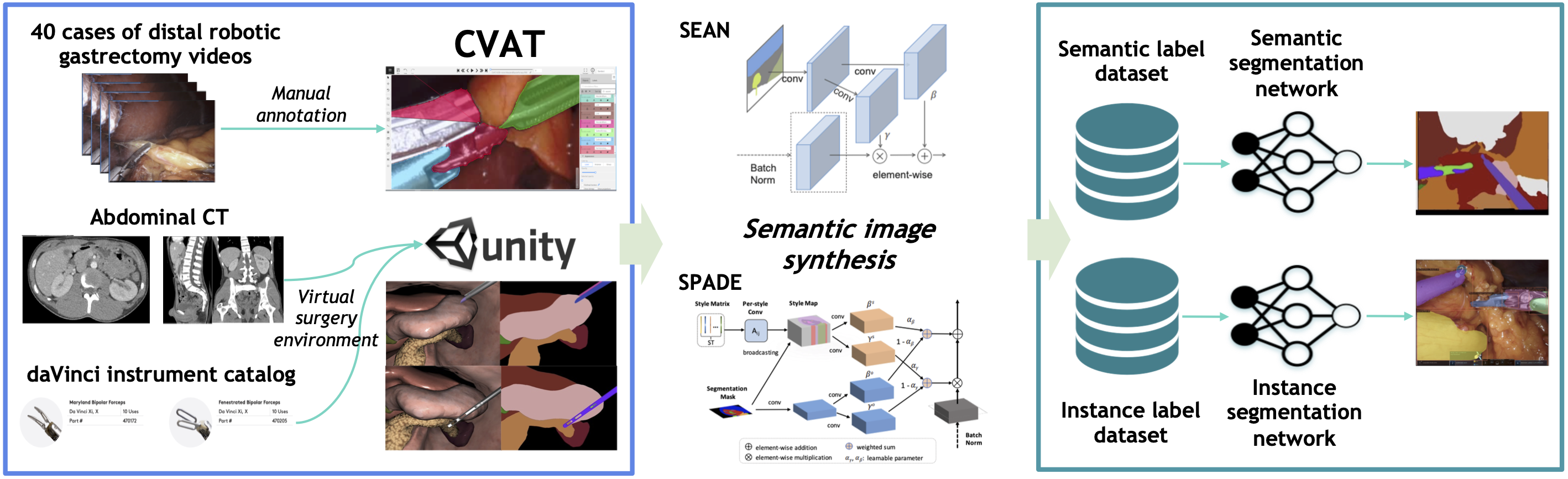
We investigated the impact of synthetic training data on instance and semantic segmentation performance. Specifically, we evaluated two categories of synthetic data—manually synthesized (MS) and domain-randomized synthetic (DRS)—using three semantic synthesis models: SPADE, SEAN, and SRC. In contrast to our previous work, we additionally explored the efficacy of the SRC model in performing unsupervised image-to-image translation to generate photo-realistic synthetic training images.

Implementation Details

We utilized MMDetection v3.2.0 [Chen et al., 2019b] and MMSegmentation v1.2.2 [MMSegmentation Contributors, 2020], built upon MMCV v1.2.0, MMEngine v0.10.3, PyTorch v2.1.2, and TorchVision v0.16.2, representing the latest available versions at the time of writing. For image synthesis, software versions were consistent with those in prior studies. Notably, updates to these major packages introduced deviations from previous findings [Yoon et al., 2022]. To ensure reproducibility and mitigate randomness-induced variability, a fixed random seed was used throughout all training and evaluation procedures.

All segmentation models incorporating real and synthetic data were trained for 40 epochs. For fairness, training epochs for models utilizing only real data were adjusted to match the total number of iterations experienced by models trained with combined real and synthetic data. The best-performing checkpoint was selected as the representative model from each training run. Synthetic data-trained models typically reached optimal performance around epoch 34, confirming no additional performance gains beyond 40 epochs. Detailed hyperparameters are provided in Table 12.

Manual synthetic (MS) data generation initially produced 3400 images. Subsequently, images containing objects (instrument head or entire instrument) below a pixel threshold of 10,900 were excluded. Applying Object Size-aware Random Crop (OSRC), we generated the MS+C dataset. OSRC utilized a fixed random seed (0) and targeted object size ratios within the median to 75th percentile range of real object distributions, determined empirically. Further refinement by reassigning the background class to "other anatomical tissues" resulted in the MS+C+B dataset. Each MS dataset variant was photo-realistically synthesized using SPADE, SEAN, and SRC models, denoted as ModelName(MS+...). These synthesized datasets were combined with real training data (R) as R+ModelName(MS+...) for subsequent training.

Domain-randomized synthetic (DRS) data production generated 4474 images. Initially applying OSRC, we then eliminated images containing objects with a size ratio below 0.0005. Using identical random seed and size distribution parameters as in MS data, the refined DRS data served as sources for copy-paste augmentation. To streamline the process, augmentation via copy-paste and subsequent photo-realistic synthesis were performed offline, with augmented images and masks stored before training. Half of the training dataset comprised augmented copy-paste (CP) data combined from real and DRS masks, and half consisted of original real data, denoted as R+ModelName(R+DRS+...+CP). For comparative analysis, we also generated a baseline dataset synthesized exclusively from real masks, labeled as R+ModelName(R+CP). Detailed statistics of domain-randomized data utilized in copy-paste augmentation are summarized in Table 11.

Relative Performance Improvement

To quantitatively measure the benefit provided by synthetic data relative to real data, we propose a metric termed Relative Performance Improvement. Specifically, the Relative performance improvement metric is defined as:

Relative Metric = (Metric_R+Syn - Metric_R) / Metric_R

where the metric can be AP, IoU, or Accuracy. By calculating this ratio, we explicitly assess the relative performance gains attributable to synthetic data augmentation, denoted as Relative AP, Relative IoU, and Relative Acc.

Instance Segmentation with Manual Synthetic Data

To quantitatively evaluate segmentation performance, we employed two state-of-the-art segmentation models, Cascade Mask R-CNN (CMR) and Hybrid Task Cascade (HTC), and assessed their bounding box and mask performance using mean average precision (box mAP and mask mAP) as defined by the MS-COCO benchmark [Lin et al., 2014]. Additionally, we calculated mean Relative Average Precision (box mRAP and mask mRAP) to explicitly measure the relative performance enhancement achieved by synthetic data augmentation compared to real data alone.

As summarized in Table 2, incorporating synthetic data consistently improved the mean box AP across both CMR and HTC models. However, mask AP improvement was less consistent. Notably, the best overall performances were achieved using the R+SPADE(MS+C+B) dataset, yielding the highest mean box AP of 54.92 and mask AP of 50.04 for CMR.

A detailed class-specific analysis in Table 3 highlights results that differ substantially from the aggregate performance. Specifically, Table 3 presents the top 10 and bottom 10 classes based on performance improvements for instrument detection using the CMR model trained on the R+SPADE(MS+C+B) dataset. This reveals significant class-specific variations, emphasizing the necessity of detailed, class-level analysis beyond aggregated metrics.

Table 2. Performance metrics (mean mAP ± standard deviation) for Cascade Mask R-CNN (CMR) and Hybrid Task Cascade (HTC) trained on manual synthetic (MS) datasets. Best performance for each model is indicated in bold.

Model	Dataset	Box mAP (Mean ± Std.)	Mask mAP (Mean ± Std.)
Cascade Mask R-CNN (CMR)	R	53.93 ± 0.98	49.75 ± 1.05
	R+SEAN(MS)	54.32 ± 1.25	49.00 ± 1.22
	R+SPADE(MS)	54.31 ± 1.43	48.98 ± 1.41
	R+SEAN(MS+C)	54.69 ± 1.19	49.46 ± 1.23
	R+SPADE(MS+C)	54.82 ± 1.38	49.58 ± 1.46
	R+SEAN(MS+C+B)	54.89 ± 0.97	49.55 ± 1.10
	R+SPADE(MS+C+B)	54.92 ± 1.04	50.04 ± 1.07
Hybrid Task Cascade (HTC)	R	55.06 ± 0.86	51.67 ± 0.56
	R+SEAN(MS)	55.55 ± 1.34	50.95 ± 1.08
	R+SPADE(MS)	55.51 ± 0.77	50.88 ± 1.05
	R+SEAN(MS+C)	56.09 ± 0.78	51.44 ± 0.97
	R+SPADE(MS+C)	56.23 ± 1.08	51.40 ± 1.22
	R+SEAN(MS+C+B)	56.20 ± 0.93	51.37 ± 1.13
	R+SPADE(MS+C+B)	56.36 ± 0.94	51.77 ± 1.04

Table 3. Relative performance improvements (%) of Cascade Mask R-CNN using synthetic data (R+SPADE(MS+C+B)) compared to real data alone across three cross-validation sets. The top 10 classes with the greatest improvement and the bottom 10 classes with the least improvement are shown.

Category (Top 10)	Real Box mAP	Relative Box mAP	Real Mask mAP	Relative Mask mAP
DT	20.90	+23.29	27.20	+5.88
ND	31.10	+18.11	6.93	-0.96
Liver	32.33	+15.15	39.07	+7.08
CAG_H	14.07	+11.37	10.47	+8.92
SB	41.70	+10.23	38.73	+4.13
GZ	34.00	+8.43	46.10	+1.81
Spleen	26.13	+7.78	30.63	+5.88
Pancreas	27.30	+7.69	27.60	+11.71
Stomach	41.83	+7.09	47.40	+4.57
S_H	57.17	+6.88	53.00	+1.51

Category (Bottom 10)	Real Box mAP	Relative Box mAP	Real Mask mAP	Relative Mask mAP
SCA_W	83.07	-0.48	83.10	-0.84
HA_B	70.43	-0.62	64.97	-1.03
CF_W	65.47	-0.81	58.27	+0.11
MLCA_B	69.33	-1.49	67.90	-2.16
S_B	42.07	-1.66	39.63	+3.36
SCA_B	82.10	-1.66	77.07	+0.74
HA_H	53.80	-1.80	32.43	-3.08
SI	73.47	-2.27	71.30	-3.04
MLCA_W	76.40	-2.79	68.30	-0.29
MLCA_H	68.20	-4.30	55.77	-2.51

Semantic Segmentation with Manual Synthetic Data

We evaluated semantic segmentation performance using two representative models, DeepLabV3+ and UperNet, employing standard metrics including mean Intersection-over-Union (mIoU) and mean Accuracy (mAcc). Additionally, we introduced mean Relative IoU (mRIoU) and mean Relative Accuracy (mRAcc) metrics, analogous to those used in our instance segmentation evaluation, to quantitatively assess improvements from synthetic data augmentation.

Table 4 summarizes semantic segmentation results across synthetic datasets. Interestingly, uncropped synthetic datasets generally outperformed cropped variants, contrasting the instance segmentation findings. Among synthetic data combinations, R+SPADE(MS+C+B) achieved the highest performance for both segmentation models. We attribute the observed lower relative improvements compared to instance segmentation to the already high baseline performance obtained with the real dataset alone (e.g., 74.63 Mean mIoU with UperNet).

A more detailed analysis of class-level performances (Table 5) for semantic segmentation using UperNet trained on R+SPADE(MS+C+B) highlights notably smaller relative gains compared to instance segmentation. This is primarily due to the already high baseline accuracy for the top-performing classes. Furthermore, unlike instance segmentation, all uncropped synthetic datasets consistently outperformed cropped ones, indicating task-dependent sensitivity to cropping strategies.

Table 4. Performance metrics (Mean ± Std.) for UperNet (UPN) and DeepLabV3+ (DLV3+) trained on manual synthetic (MS) datasets across three cross-validation datasets. Best performance for each model is indicated in bold.

Model	Dataset	Mean mIoU (± Std.)	Mean mAcc (± Std.)
UperNet (UPN)	R	74.63 ± 1.04	83.35 ± 0.86
	R+SEAN(MS)	72.87 ± 0.77	82.10 ± 0.87
	R+SPADE(MS)	73.42 ± 0.90	82.60 ± 0.72
	R+SEAN(MS+C)	72.74 ± 0.97	82.05 ± 0.69
	R+SPADE(MS+C)	73.16 ± 1.32	82.49 ± 1.10
	R+SEAN(MS+C+B)	72.44 ± 0.90	81.93 ± 0.65
	R+SPADE(MS+C+B)	72.60 ± 1.25	81.99 ± 0.89
DeepLabV3+ (DLV3+)	R	74.62 ± 0.84	83.65 ± 0.74
	R+SEAN(MS)	72.71 ± 0.90	82.10 ± 0.65
	R+SPADE(MS)	73.18 ± 0.97	82.53 ± 0.93
	R+SEAN(MS+C)	72.04 ± 1.31	81.84 ± 1.26
	R+SPADE(MS+C)	72.56 ± 1.30	82.14 ± 1.10
	R+SEAN(MS+C+B)	71.70 ± 0.78	81.62 ± 0.87
	R+SPADE(MS+C+B)	72.07 ± 0.86	81.81 ± 0.94

Table 5. Relative performance improvements (%) for UperNet trained on R+SPADE(MS) compared to the R dataset across three cross-validation datasets. The top 10 and bottom 10 classes based on mean IoU (mIoU) are listed.

Category (Top 10)	Real Mean mIoU	Relative Mean mIoU (%)	Real Mean mAcc	Relative Mean mAcc (%)
Spleen	31.23	+3.10	35.65	+3.73
Pancreas	56.54	+1.73	69.04	+1.50
Gallbladder	59.93	+0.91	66.01	+2.06
Stomach	67.03	+0.26	84.97	+0.36
SCA_B	80.75	+0.14	86.37	+0.34
TO_T	82.85	-0.06	92.26	-0.42
GZ	92.96	-0.20	96.41	0.00
ET	91.69	-0.27	97.69	-0.13
Liver	78.33	-0.28	87.50	+0.38
SCA_W	88.27	-0.42	93.49	-0.07

Category (Bottom 10)	Real Mean mIoU	Relative Mean mIoU (%)	Real Mean mAcc	Relative Mean mAcc (%)
MBF_B	73.83	-2.46	84.21	-2.49
SCA_H	84.40	-2.79	84.42	-2.27
S_H	81.78	-2.93	89.56	-0.35
SI	75.20	-3.08	81.52	-2.51
ND	57.32	-3.39	69.86	-2.54
CF_W	76.53	-3.60	87.67	-2.60
MLCA_H	79.54	-4.08	89.39	-1.72
HA_H	65.67	-4.33	78.38	-2.60
S_B	78.43	-4.93	85.67	-3.47
CAG_H	41.10	-7.40	52.22	-3.04

Domain Randomized Synthetic Data

Tables 6 and 7 summarize results obtained using domain-randomized synthetic (DRS) data as a source for copy-paste (CP) augmentation across segmentation models. Our results demonstrate that DRS-based copy-paste consistently improves performance for instance segmentation models, as evidenced by increased box and mask AP scores. However, when extending this augmentation method to semantic segmentation, no performance gains were observed. We hypothesize that the lack of improvement in semantic segmentation models is primarily due to their already strong baseline performance with real data, limiting the potential effectiveness of the additional synthetic augmentation.

Table 6. Performance metrics (Mean ± Std.) of Cascade Mask R-CNN (CMR) and Hybrid Task Cascade (HTC) trained using domain-randomized synthetic (DRS) datasets combined with the copy-paste (CP) augmentation strategy across three cross-validation datasets. Best results are highlighted in bold.

Model	Dataset	Box Mean mAP (± Std.)	Mask Mean mAP (± Std.)
Cascade Mask R-CNN (CMR)	R+SPADE(R+CP)	58.09 ± 0.91	50.86 ± 1.06
	R+SPADE(R+DRS+C+B+CP)	58.18 ± 0.67	51.10 ± 0.97
Hybrid Task Cascade (HTC)	R+SPADE(R+CP)	59.68 ± 0.65	52.96 ± 0.89
	R+SPADE(R+DRS+C+B+CP)	59.68 ± 0.75	52.95 ± 0.96

Table 7. Performance metrics (mean ± std.) for UperNet (UPN) and DeepLabV3+ (DLV3+) models using copy-paste augmentation with Domain Randomized Synthetic (DRS) dataset. Metrics are averaged over three cross-validation datasets. Best results are highlighted in bold.

Model	Dataset	Mean mIoU (± Std.)	Mean mAcc (± Std.)
UperNet (UPN)	R+SPADE(R+CP)	70.26 ± 1.08	80.17 ± 0.78
	R+SPADE(R+DRS+C+B+CP)	70.08 ± 0.99	80.02 ± 0.74
DeepLabV3+ (DLV3+)	R+SPADE(R+CP)	72.39 ± 4.05	82.31 ± 3.15
	R+SPADE(R+DRS+C+B+CP)	69.46 ± 1.02	79.88 ± 0.85

Real Data Size vs. Synthetic Data Effectiveness

Tables 8 and 9 present segmentation results obtained using a reduced-size real dataset (R1(H), half-sized dataset for cross-validation set 1) combined with a full-scale synthetic dataset. Unlike previous results shown in Table 2, where the CMR model achieved the best performance using SPADE(MS+C+B), here the highest improvement in mAP was obtained with SPADE(MS+C) data. Interestingly, despite a reduced real-data baseline, semantic segmentation models (UperNet and DeepLabV3+) maintained robust performance (~71 mIoU) even without synthetic augmentation, and thus no overall improvements were observed when incorporating synthetic data. This indicates semantic segmentation models are less sensitive to synthetic data augmentation in scenarios with moderately reduced training data. Future work will further investigate scenarios with significantly smaller real training datasets.

Table 8. Performance metrics (box mAP and mask mAP) for Cascade Mask R-CNN (CMR) and Hybrid Task Cascade (HTC) trained on Manual Synthetic (MS) datasets combined with half-sized real data (H). The highest performance per model is highlighted in bold.

Model	Dataset	Box mAP	Mask mAP
Cascade Mask R-CNN (CMR)	R1(H)	49.14	44.38
	R1(H)+SEAN(MS)	49.36	43.19
	R1(H)+SPADE(MS)	50.74	44.04
	R1(H)+SEAN(MS+C)	50.51	44.45
	R1(H)+SPADE(MS+C)	51.40	44.93
	R1(H)+SEAN(MS+C+B)	50.78	44.61
	R1(H)+SPADE(MS+C+B)	51.35	44.86
Hybrid Task Cascade (HTC)	R1(H)	51.02	45.38
	R1(H)+SEAN(MS)	51.40	45.93
	R1(H)+SPADE(MS)	51.31	45.65
	R1(H)+SEAN(MS+C)	51.96	46.44
	R1(H)+SPADE(MS+C)	52.39	46.71
	R1(H)+SEAN(MS+C+B)	52.65	46.90
	R1(H)+SPADE(MS+C+B)	52.76	46.73

Table 9. Performance metrics (mIoU and mAcc) for UperNet (UPN) and DeepLabV3+ (DLV3+) trained on manual synthetic (MS) datasets combined with half-sized real data (H). Metrics are averaged over three cross-validation datasets. The highest performance per model is highlighted in bold.

Model	Dataset	mIoU (%)	mAcc (%)
UperNet (UPN)	R1(H)	71.74	80.97
	R1(H)+SEAN(MS)	69.03	79.04
	R1(H)+SPADE(MS)	68.60	78.78
	R1(H)+SEAN(MS+C)	66.95	77.34
	R1(H)+SPADE(MS+C)	68.38	78.32
	R1(H)+SEAN(MS+C+B)	65.58	76.25
	R1(H)+SPADE(MS+C+B)	67.31	77.39
DeepLabV3+ (DLV3+)	R1(H)	71.77	81.04
	R1(H)+SEAN(MS)	68.28	78.82
	R1(H)+SPADE(MS)	68.23	78.69
	R1(H)+SEAN(MS+C)	65.78	76.96
	R1(H)+SPADE(MS+C)	67.03	77.67
	R1(H)+SEAN(MS+C+B)	65.74	76.73
	R1(H)+SPADE(MS+C+B)	66.17	77.09

Semantic Image Synthesis

We evaluated the effectiveness of synthetic data generated by the SPADE and SEAN models for training both instance and semantic segmentation networks. To quantitatively assess image synthesis quality, we adopted the three-step evaluation framework proposed by Park et al. 2019 and Zhu et al., 2020: (1) segmentation models were trained solely on real data; (2) segmentation models were evaluated on both real validation data and corresponding synthesized validation sets produced by SPADE and SEAN; (3) the segmentation performance on original and synthesized validation sets was directly compared.

Table 10 presents the evaluation results on photo-realistic synthesized validation sets as well as the average mAP achieved when training segmentation models with synthetic datasets from each synthesis method. While both SPADE and SEAN produced high-quality photo-realistic data, SEAN achieved superior validation set fidelity across most metrics. However, in terms of overall synthetic training data effectiveness (average mAP), SPADE-generated datasets provided comparable or slightly higher improvements, suggesting a task-dependent distinction between visual realism and segmentation model performance.

Table 10. Performance metrics for evaluating the photo-realistic synthesis abilities of SPADE and SEAN models. "AVG Syn" indicates the average segmentation model performance trained with SPADE/SEAN-generated synthetic datasets (MS/F/C/B) evaluated on the R1-valid dataset.

Model	Train/Valid	mAP/mIoU	mAP/mAcc	AVG Syn mAP/mIoU	AVG Syn mAP/mAcc
Cascade Mask R-CNN (CMR)	R1/R1-valid	0.543	0.497	–	–
	R1/SEAN(R1-valid)	0.472	0.437	55.25	49.33
	R1/SPADE(R1-valid)	0.411	0.373	55.00	49.43
Hybrid Task Cascade Mask R-CNN (HTC)	R1/R1-valid	0.555	0.516	–	–
	R1/SEAN(R1-valid)	0.486	0.453	56.38	51.10
	R1/SPADE(R1-valid)	0.431	0.398	56.15	51.05
UperNet (UPN)	R1/R1-valid	73.73	87.87	–	–
	R1/SEAN(R1-valid)	60.35	83.69	71.87	81.29
	R1/SPADE(R1-valid)	58.30	83.92	72.47	81.85
DeepLabv3+ (DLV3+)	R1/R1-valid	88.10	74.05	–	–
	R1/SEAN(R1-valid)	62.77	73.73	71.67	81.28
	R1/SPADE(R1-valid)	60.73	71.54	71.98	81.33

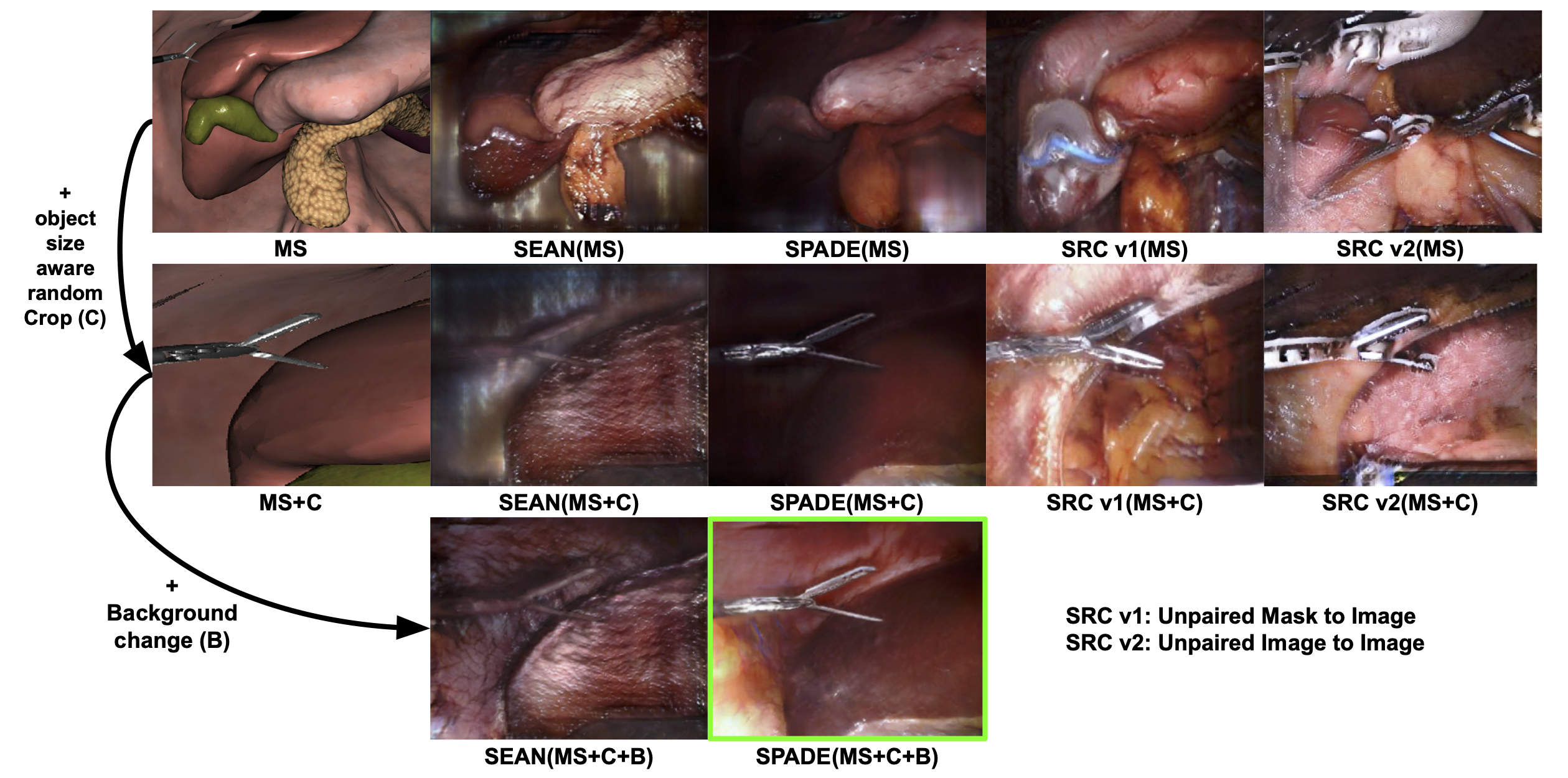
Qualitative Analysis of Synthetic Data

Figure 2 qualitatively illustrates improvements toward photo-realistic synthesis by sequentially applying Object Size-aware Random Crop (OSRC) and Background Label Enhancement. The initial synthetic images (first row) differ considerably from real surgical scenes, complicating realistic image generation. Applying OSRC (second row) effectively aligns object sizes with real distributions, yet unnatural background textures remain. Subsequently, introducing Background Label Enhancement (third row) significantly removes these unnatural artifacts, resulting in images closely resembling actual surgical scenes. Notably, although SEAN exhibits the best quantitative performance with real validation masks (Table 11), this may indicate model sensitivity or potential overfitting to real data distributions.

Unsupervised Image Translation

We compared the effectiveness of unsupervised image translation (SRC) and supervised semantic image synthesis methods (SPADE and SEAN) for generating photo-realistic synthetic data, as illustrated in Figure 2. Two SRC variants were explored: one trained to translate real segmentation masks into real images (analogous to supervised synthesis methods), and the other directly translating synthetic masks to realistic images. Qualitative results revealed that both SRC models failed to adequately capture semantic consistency, producing unnatural synthesis outcomes. We hypothesize that the substantial domain gap between synthetic and real data prevents the SRC models from accurately learning semantic relationships, resulting in inferior synthesis quality. Despite its advantage of not requiring labeled pairs, SRC's effectiveness may be significantly limited when the domain discrepancy is large, highlighting challenges for unsupervised translation in this setting.

Table 11. Class distribution and number of frames per dataset. Each cross-validation set includes Real# and Test#. Manual synthetic data (MS) and domain randomized synthetic data (DRS) are identical across all cross-validation sets. (HA: Harmonic Ace, CF: Cadiere Forceps, MBF: Maryland Bipolar Forceps, MCA: Medium-large Clip Applier, SCA: Small Clip Applier, CAG: Curved Atraumatic Grasper, DT: Drain Tube, OI: other instruments, OT: other tissues, H: head, W: wrist, B: body)

Category	R1	R1-valid	R2	R2-valid	R3	R3-valid	MS	MS+F	MS+F+C(B)	DRS+F+C
HA H	1317	450	1304	463	1305	462	289	284	523	262
HA B	1268	448	1285	431	1272	444	297	286	528	261
MBF H	1460	486	1451	495	1439	507	297	292	582	425
MBF W	1092	376	1132	336	1060	408	286	285	1705	425
MBF B	672	256	724	204	679	249	273	273	514	402
CF H	1093	338	1058	373	1045	386	515	490	611	110
CF W	900	258	842	316	856	302	441	425	831	108
CF B	854	271	816	309	831	294	407	396	498	103
CAG H	704	231	687	248	705	230	692	690	2884	78
CAG B	787	269	779	277	803	253	691	688	1790	77
S H	329	111	322	118	335	105	293	292	436	560
S B	305	98	297	106	301	102	298	292	401	560
MLCA H	287	95	282	100	291	91	300	297	1314	387
MLCA W	230	82	233	79	236	76	299	297	554	386
MLCA B	140	50	142	48	141	49	287	287	405	370
SCA H	277	85	266	96	276	86	300	299	322	156
SCA W	261	78	247	92	258	81	300	299	505	156
SCA B	183	51	179	55	175	59	299	299	460	138
SI	286	92	273	105	286	92	298	297	297	758
ND	303	115	322	96	306	112	299	287	999	177
DT	298	97	296	99	297	98	300	299	301	794
SB	506	145	484	167	449	202	300	300	729	0
DT	308	103	284	127	299	112	3243	3168	2250	767
Liver	2785	913	2745	953	2741	957	3399	3322	3168	0
Stomach	2278	776	2286	768	2336	718	3264	3187	2603	0
Pancreas	1507	574	1544	537	1623	458	3115	3048	2131	0
Spleen	338	172	422	88	373	137	2232	2163	1063	0
Gallbladder	816	353	935	234	916	253	0	0	0	0
GZ	2705	942	2692	955	2707	940	0	0	0	0
TO I	1569	552	1571	550	1654	467	0	0	0	0
TO T	3367	1135	3352	1150	3370	1132	0	0	0	0
Frames	3375	1135	3355	1155	3377	1133	3400	3322	3318	4474

Table 12: Hyper-parameters for Semantic Image Synthesis and Segmentation Models.
(a) Semantic image synthesis: Both SPADE and SEAN employ the hinge loss with identical hyper-parameter settings (λ_feat = 10.0, λ_kld = 0.005, λ_vgg = 10.0), and their generator (G) and discriminator (D) architectures follow the original implementations. Batch size (BS) and augmentation strategies are also provided.
(b) Segmentation: Hyper-parameters for DLV3+, UperNet, Cascade Mask R-CNN (CMR), and Hybrid Task Cascade (HTC) are listed. Here, β denotes momentum, weight decay (WD) and initial learning rate (LR) are specified along with the LR scheduler (indicating scaling epochs with a factor of 0.1), batch size (BS), and warmup (WU) parameters. All backbones are pre-trained on the ImageNet dataset.

(a) Hyper-parameters for Semantic Image Synthesis Models

Method	D step per G	Input size	Optimizer	Beta	Init. LR	Final epoch	BS	Augmentation
SPADE	1	512x512	Adam	β₁=0.5, β₂=0.999	4×10⁻⁴	50	20	resize, crop, flip
SEAN	1	512x512	Adam	β₁=0.5, β₂=0.999	2×10⁻⁴	100	8	resize, flip

(b) Hyper-parameters for Segmentation Models

Method	Backbone	Input size	Optimizer	Init. LR	LR scheduler (final)	BS	WU (iter)	WU (ratio)
DLV3+	ResNet 101	512x512	SGD	0.001	cos. annealing (300)	8	1000	0.1
UperNet	ResNet 101	512x512	AdamW	6×10⁻⁴	Poly (300)	8	1500	1.0×10⁻⁶
CMR	ResNet101	1333x800	SGD	0.02	step [32] (34)	16	1000	0.002
HTC	ResNet101	1333x800	SGD	0.02	step [32] (34)	16	1000	0.002

Conclusion

We presented SISVSE, a large-scale surgical segmentation dataset that combines real annotated images from robotic distal gastrectomy with diverse, automatically annotated synthetic data. Our novel Virtual Surgery Environment enables the generation of anatomically accurate 3D scenes by incorporating patient-derived CT scans and precisely measured surgical instruments, thus mitigating the need for extensive manual annotations. To bridge the remaining domain gap, we proposed Object Size-Aware Random Crop (OSRC) and Background Label Enhancement, significantly improving the realism of photo-realistic semantic image synthesis. Through comprehensive experiments on state-of-the-art segmentation models, we demonstrated that these synthetic data augmentations yield notable gains in instance segmentation performance—particularly for challenging or low-frequency classes—and also maintain competitive results in semantic segmentation. Our exploration of domain-randomized synthetic data for copy-paste augmentation further underscores the potential of synthetic data in surgical AI, even though improvements in semantic segmentation proved less substantial compared to instance segmentation. augmentations yield notable gains in instance segmentation performance—particularly for challenging or low-frequency classes—and also maintain competitive results in semantic segmentation. Our exploration of domain-randomized synthetic data for copy-paste augmentation further underscores the potential of synthetic data in surgical AI, even though improvements in semantic segmentation proved less substantial compared to instance segmentation.

By making SISVSE and our methodology publicly available, we aim to accelerate research in robotic and laparoscopic surgery, reduce the reliance on scarce manually annotated datasets, and inspire future developments in synthetic data generation and domain adaptation. Beyond gastrectomy, our approach is readily extensible to other clinical procedures requiring robust image segmentation under limited supervision. We hope this work fosters new opportunities for data-efficient training paradigms, opens avenues for more realistic synthetic-to-real translations, and ultimately contributes to safer, more advanced computer-assisted surgery.

References

Chen, K., Wang, J., Pang, J., et al. (2019). MMDetection: Open mmlab detection toolbox and benchmark. arXiv preprint arXiv:1906.07155.

Intel Corporation (2019). Computer Vision Annotation Tool (CVAT). https://github.com/opencv/cvat

Jung, C., Kwon, G., & Ye, J.C. (2022). Exploring patch-wise semantic relation for contrastive learning in image-to-image translation tasks. In Proceedings of CVPR.

Lin, T.Y., Maire, M., Belongie, S., et al. (2014). Microsoft COCO: Common objects in context. In Proceedings of ECCV.

MMSegmentation Contributors (2020). MMSegmentation: OpenMMLab semantic segmentation toolbox and benchmark. https://github.com/open-mmlab/mmsegmentation

Park, T., Liu, M.Y., Wang, T.C., & Zhu, J.Y. (2019). Semantic image synthesis with spatially-adaptive normalization. In Proceedings of CVPR.

Schroeder, W., Martin, K., & Lorensen, B. (2006). The Visualization Toolkit: An Object-Oriented Approach to 3D Graphics (4th ed.). Kitware.

Tremblay, J., Prakash, A., Acuna, D., et al. (2018). Training deep networks with synthetic data: Bridging the reality gap by domain randomization. In Proceedings of CVPR Workshops.

Yoon, Y., Choi, W., Han, D.M., et al. (2020). Semi-supervised learning for instrument detection with a class imbalanced dataset. In Proceedings of MICCAI Workshops.

Yoon, J., Hong, S., Lee, J., et al. (2022). Surgical scene segmentation using semantic image synthesis with a virtual surgery environment. In Proceedings of MICCAI.

Zhu, X., Hu, H., Lin, S., & Dai, J. (2020). SEAN: Image synthesis with semantic region-adaptive normalization. In Proceedings of CVPR.

Citation

If you find our work useful in your research, please consider citing:

@misc{yoon2024sisvseenhanced,
  title={Surgical Scene Segmentation Using Semantic Image Synthesis with a Virtual Surgery Environment: Enhanced with Object Size-Aware Random Crop and Background Label Enhancement for Photo-Realistic Synthesis},
  url={https://sisvse.github.io/},
  author={Jihun Yoon, Bogyu Park, Jiwon Lee, Bokyung Park, Sungjae Kim, SungHyun Park, Woo Jin Hyung, and Min-Kook Choi},
  month={March},
  year={2024}
}

SISVSE

Surgical Scene Segmentation Using Semantic Image Synthesis with a Virtual Surgery Environment

Enhanced with Object Size-Aware Random Crop and Background Label Enhancement for Photo-Realistic Synthesis

Overview

Introduction

Contribution

SISVSE: A Large-Scale Surgical Segmentation Dataset

Virtual Surgery Environment for Data Generation

Photo-Realistic Semantic Image Synthesis

Object Size-Aware Random Crop (OSRC)

Background Label Enhancement

Comprehensive Evaluation on Segmentation Models

Open Platform for Future Surgical AI Research

Methodology

Real Surgery Data Curation

Categories

Class-Balanced Frame Sampling

Virtual Surgery Environment and Synthetic Data

High-Quality Annotations for Real and Synthetic Data

Semantic Image Synthesis

Object Size-Aware Random Crop (OSRC)

Background Label Enhancement

Experiments

Implementation Details

Relative Performance Improvement

Instance Segmentation with Manual Synthetic Data

Semantic Segmentation with Manual Synthetic Data

Domain Randomized Synthetic Data

Real Data Size vs. Synthetic Data Effectiveness

Semantic Image Synthesis

Qualitative Analysis of Synthetic Data

Unsupervised Image Translation

Conclusion

References

Citation